Global upper-atmospheric heating on Jupiter by the polar aurorae

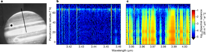
Jupiter was observed with the 10-m Keck II telescope for five hours on both 14 April 2016 and 25 January 2017 using NIRSPEC (Near-InfraRed Spectrometer¹⁴), with the spectral slit aligned north–south along the axis of planetary rotation (Fig. 1a). Spectral images were acquired as Jupiter rotated, as shown in Fig. 1b, c, in which rotational–vibrational (ro-vibrational) emission lines of the H₃⁺ ion can be seen extending from pole to equator. These ions are a major constituent of Jupiter’s ionosphere and mainly reside in the altitude range 600–1,000 km above the 1-bar pressure surface¹⁵. The intensity ratio of two or more H₃⁺ lines can be used to derive the column-averaged parameters of that ion: temperature, number density and radiance¹⁶. As H₃⁺ is assumed to be in quasi-local thermodynamic equilibrium with Jupiter’s upper atmosphere¹⁶, its derived temperature is representative of the region. Details of the H₃⁺ fitting process and global mapping of parameters are provided in the Methods and in Extended Data Figs. 1, 2.

a, Slit-viewing camera image filtered between 2.134 μm and 4.228 μm wavelength. Guide images such as this are taken every 9 s and indicate the slit’s position on the sky relative to Jupiter. In this image, the Great Red Spot (bottom left) and satellite Ganymede (top left) can be seen. b, c, Spectral images of Jupiter showing spectral radiance as a function of wavelength and planetocentric latitude. Most emissions seen in c are from the reflection of sunlight from hydrocarbons and hazes. Well-defined vertical lines are H₃⁺ ro-vibrational emission lines: they are most intense in the polar regions. The R(3,0) and Q(1,0) H₃⁺ lines at 3.41277 μm and 3.9529 μm are the focus of this study, as their consistently high signal-to-noise (SNR) at all latitudes allows us to map upper-atmospheric energy balance globally. The SNR of H₃⁺ is high at Jupiter owing to the convenient presence of a deep methane absorption band, particularly in b (ref. ²⁷).

Full size image

Global maps of upper-atmospheric temperature have been produced previously¹⁷, but the spatial resolution was such that about two pixels covered 45–90° latitude in each hemisphere, making it difficult to assess how the auroral region was connected to the rest of the planet. In those maps, equatorial temperatures were similar to auroral values, a finding that would indicate that a heat source is active at low latitudes. In Figs. 2 and 3, we show near-global maps of Jovian column-averaged H₃⁺ temperature, density and radiance, which are the product of several thousand individual fits to the spectral data (see Methods). Using a magnetic field model, we have overlaid oval-shaped lines on the polar regions of Jupiter in both Figs. 2 and 3, with each representing the footprint of magnetic field lines that trace from the planet out to a particular distance in Jupiter’s equatorial plane¹⁸. The main (auroral) oval traces on average to 30R_J in Jupiter’s equatorial plane (R_J is Jupiter’s equatorial radius of 71,492 km at the 1-bar pressure level). The satellite footprints of Io and Amalthea are fiducial markers, mapping out from the planet to 5.9R_J and 2.54R_J in the equatorial plane, respectively.

Projections are shown as a function of central meridian longitude (Jovian system III) and planetocentric latitude. Temperature (T) and radiance (E) panels have uncertainties below 5%, while column densities (N) are limited to 20%. Long black-and-white dashed lines show Jupiter’s main auroral oval, short black-and-white dashed lines correspond to the magnetic footprint of Io, and the single thick black line corresponds to the magnetic footprint of Amalthea (described in the main text). White indicates regions with no data coverage (or where no results met the uncertainty criteria). Median (and maximum) uncertainty percentiles for 14 April 2016 are: temperature 2.2% (5%), density 9.4% (15%) and radiance 2.2% (5%). Median (and maximum) uncertainties for 25 January 2017 are: temperature 1.6% (5%), density 5.8% (15%) and radiance 1.8% (5%). The Methods describes the mapping process, and Extended Data Tables 1–3 show the bin sizes that were used in each parameter map.

Full size image

a, Orthographic projections of uncertainties in temperature are all below 5%. Long black-and-white dashed lines show Jupiter’s main auroral oval, short black-and-white dashed lines correspond to the magnetic footprint of Io, and the single thick black line corresponds to the magnetic footprint of Amalthea (as described in the main text). A visible computer-generated globe of Jupiter based on Hubble Space Telescope imagery is shown underneath the H₃⁺ temperature projection. Image credit: NASA Goddard Space Flight Center and the Space Telescope Science Institute. Note that Jupiter is tilted differently on each date to reveal different features. The longitude and latitude gridlines shown are spaced in 60° and 10° increments, respectively. Median (and maximum) uncertainty percentiles are 2.2% (5%) for 14 April 2016 and 1.6% (5%) for 25 January 2017. b, Median Jovian H₃⁺ temperatures found for each latitude across all longitudes. Error bars are 1σ and indicate the variation of temperature over all longitudes. The Methods describes the mapping process, and Extended Data Table 1 shows the spatial bin sizes that were used in each projection.

Source data.

Full size image

Temperatures generally decrease from 1,000 K to 600 K between auroral latitudes and the equator, as shown in Figs. 2 and 3. Densities of H₃⁺, which are enhanced by aurorally driven charged-particle precipitation^19,20, cut off sharply near the main oval on both dates, indicating that the direct influence of the aurora ends within several degrees of the main oval. At the same time, equatorward of the auroral regions, H₃⁺ temperatures do not sharply fall with latitude. In the absence of any known sub-auroral electric current systems (as are common on Earth²¹) provided through magnetosphere–ionosphere coupling that cause planetary-scale ion–neutral collisions, we interpret the observed temperature gradients as strong evidence that the auroral upper atmosphere is migrating away from the auroral region to lower latitudes and adjacent longitudes, transporting its heat signature along with it. This must then be enabled principally by equatorward-propagating meridional winds.

The Jovian magnetosphere, which is subjected to the solar wind, compresses in response to high dynamic pressure exerted the solar wind²². One model has shown that magnetospheric compression events could lead to propagation of heat away from the main auroral oval towards the equator and polar cap, introducing a temporary local temperature increase of 50–175 K (refs. ^10,23). Temperatures were higher planet-wide on 25 January, as were main oval H₃⁺ densities, so a solar wind propagation model²⁴ was used to examine the solar wind dynamic pressure and other parameters at Jupiter near the dates of our observations. It was found that dynamic pressures were over an order of magnitude higher within a day of the 25 January observations, relative to quiet conditions, and almost three times higher than conditions on 14 April. This is indicated in Extended Data Figs. 3–5 (along with increased activity in other parameters). Total auroral power has previously been found to correlate positively with the duration of quiet solar wind conditions before a solar wind compression²², so, given the much longer, quieter period of solar wind activity before the 25 January observations reported here (relative to 14 April), we expect that auroral energy deposition was larger on 25 January. Factoring in the uncertainty of the arrival time of the modelled solar wind at Jupiter, ±1 days on 14 April and ±1.5 days on 25 January, we conclude that Jupiter was observed to be in the middle of a global heating event owing to solar wind compression of the Jovian magnetosphere on 25 January.

An unusual high-temperature structure was found on 25 January equatorward of the main auroral oval, extending for 160° longitude. Here, relatively cold (~800 K) atmosphere is surrounded by hot auroral and sub-auroral atmosphere at ~1,000 K. The structure appears to straddle the fiducial footprint of Amalthea, a region mapping to Jupiter’s equatorial plane at 2.5R_J via the magnetic field, but there are no known substantial sources of plasma or current systems linking those regions. It is possible that the structure is a large region of heated upper atmosphere, caught propagating equatorward away from the main auroral oval after a ‘pulse’ in solar wind pressure was exerted on the magnetosphere¹⁰. If a heated wave of atmosphere propagates equatorward from the main auroral oval at similar velocity over all longitudes, it is likely to retain the main oval shape along the way; thus the apparent alignment of the feature with Amalthea may be circumstantial. Here we provide a simple equatorward velocity estimate to examine whether the feature’s propagation is realistic. We use the latitude separation between the structure’s centre and the main oval, which grows with longitude and therefore with time, since the data are recorded in order of increasing longitude. Equatorward velocities for the hot feature were evaluated between 180° and 260° longitude in steps of 20° longitude, with ~33 min of time elapsing between each step owing to planetary rotation. A median velocity of 620 m s⁻¹ was calculated, with minima and maxima of 500 m s⁻¹ and 1,500 m s⁻¹, respectively. These velocities are similar to equatorward-propagating travelling ionospheric disturbances observed in Earth’s ionosphere (300–1,000 m s⁻¹)²⁵ but much higher than equatorward velocities reported at Saturn (up to 100 m s⁻¹)²⁶ and modelled for Jupiter (~180 m s⁻¹)^6,10.

In the vicinity of the main oval, H₃⁺ temperatures and densities are found to anticorrelate. This may be due to charged particles having higher average precipitation energies here relative to other regions, and so penetrating deeper, producing H₃⁺ at lower, colder altitudes, or evidence that H₃⁺ is efficiently cooling the atmosphere through infrared emissions^20,27. Indeed, this may explain how the main oval appears relatively colder relative to adjacent regions, despite the fact the region may have been recently heated by hot structure as it passed by. Alternatively, the hot structure may have been triggered by an event that lasted a short period of time, sending a single wave of hot atmosphere towards the equator, while the main oval returned to relatively quiet conditions. Morphological differences between the aurorae on each date indicate the location and depth of auroral precipitation, which is reflected in the derived parameters, as reported by previous observations^19,20. The median column-integrated H₃⁺ densities on 14 April and 25 January between the equator and 30° north were 4 × 10¹⁵ m⁻² and 2 × 10¹⁵ m⁻², respectively, with the latter being similar to previous values¹⁷. The F_10.7 index, an indicator of solar activity via 10.7-cm radio emissions, was 111.8 solar flux units (SFU) and 82.5 SFU on these dates—that is, 36% larger on 14 April, explaining in part this H₃⁺ density difference. Note that retrieved H₃⁺ column densities here are expected to be lower by 20% or more of their true value, owing to temperature and density gradients in the upper atmosphere²⁷; thus differences in vertical gradients may also contribute to the measured density difference. Radiance maps indicate the degree to which H₃⁺ radiatively cools the upper atmosphere, and radiance positively correlates with both temperature and density.

Temperature gradients should reveal the dominant heat sources in Jupiter’s upper atmosphere, with wave heating showing localized low-latitude peaks¹², and auroral heating showing a monotonic fall from aurora to equator. The gradients presented here are consistent with the latter, at least on these two observed dates. Therefore, the Coriolis forces and other effects that are simulated to confine auroral energy to the magnetic polar regions are evidently overcome at Jupiter. One general circulation model appeared to redistribute auroral heat successfully at Jupiter⁶, but subsequent models did not replicate the finding, so the process that allows meridional transport remains unclear^9,10. At Saturn, latitude–altitude temperature profiles also show a negative gradient from the aurora to lower latitudes²⁶, while a recent Saturn model presents a possible mechanism to disrupt the trapping of heat in the polar regions there²⁸. Main auroral oval H₃⁺ densities and global H₃⁺ temperatures were much lower on 14 April than on 25 January, potentially in agreement with model projections²⁴ that the solar wind dynamic pressure on the Jovian magnetosphere was highest on the latter date, increasing the rates of auroral particle precipitation and global heating¹⁰. The observations on 25 January also revealed, by chance, a planetary-scale heated structure, which may be propagating away from the main auroral oval in response to a solar wind compression of the magnetosphere, or may originate in the inner magnetosphere via an unknown mechanism.